Time-dependent reliability block diagrams (RBDs) take reliability modeling to the next level. They do not just show structure. Instead, they show how reliability changes over time. That shift matters. Many real-world systems degrade, wear out, or improve with maintenance. Static RBDs miss that behavior. Time-dependent RBDs capture it.
This guide explains how they work. It also shows how to use them in Six Sigma projects. You will see formulas, tables, and practical examples. By the end, you will know how to model reliability as a function of time and use that insight to drive better decisions.
- What Is a Time-Dependent RBD?
- Why Time Matters in Reliability
- Core Concept: Reliability as a Function of Time
- Time-Dependent RBD Structures
- Example: Series System Over Time
- Example: Parallel System Over Time
- How Time-Dependent RBDs Fit into Six Sigma
- Building a Time-Dependent RBD Step by Step
- Example: Manufacturing Line
- Time-Dependent Availability vs Reliability
- Maintenance Strategies Using Time-Dependent RBDs
- Sensitivity Analysis
- Common Pitfalls
- Advanced Concepts
- Practical Example: Data Center Power System
- Software Tools
- When to Use Time-Dependent RBDs
- Benefits in Six Sigma Projects
- Example: Cost of Poor Reliability
- Linking to COPQ (Cost of Poor Quality)
- Conclusion
What Is a Time-Dependent RBD?
Time-dependent reliability block diagrams (RBDs) extend a standard reliability block diagram by including time in the model. Each block no longer has a single reliability value. Instead, each block has a reliability function.

That function looks like this:
- R(t) = probability the component survives up to time t
So, instead of saying “this component is 95% reliable,” you say:
- “This component has 95% reliability at 1,000 hours”
- “This component has 80% reliability at 5,000 hours”
That difference changes everything.
Why Time Matters in Reliability
Systems rarely fail randomly forever. Failure rates change. Components often follow patterns:
- Early failures (infant mortality)
- Random failures (useful life)
- Wear-out failures (end of life)
Because of that, reliability depends on time. Ignoring time leads to wrong conclusions.
Example
Imagine two pumps:
| Pump | Reliability at 1,000 hrs | Reliability at 5,000 hrs |
|---|---|---|
| A | 95% | 60% |
| B | 90% | 85% |
At first glance, Pump A looks better. However, over time, Pump B outperforms it. A static RBD would miss that insight.
Core Concept: Reliability as a Function of Time
Every block in a time-dependent RBD uses a reliability function.
Common Models
| Model | Formula | Use Case |
|---|---|---|
| Exponential | R(t) = e^(-λt) | Constant failure rate |
| Weibull | R(t) = e^(-(t/η)^β) | Aging or wear-out |
| Lognormal | Complex | Fatigue, crack growth |
The Weibull model dominates in Six Sigma work. It handles early failures and wear-out well.
Time-Dependent RBD Structures
The structure stays the same as traditional RBDs. However, calculations now use functions.
Series System

All components must work.
- System fails if one fails
System reliability:
Rsystem(t) = R1(t) × R2(t) × … × Rn(t)
Parallel System

At least one component must work.
- System survives if one survives
System reliability:
Rsystem(t) = 1 – [(1 – R₁(t)) × (1 – R₂(t)) × … × (1 – Rn(t))]
Mixed Systems

Most real systems combine both.
Example: Series System Over Time
Consider a system with two components:
- Component A: R₁(t) = e(-0.001t)
- Component B: R₂(t) = e(-0.002t)
System reliability:
Rsystem(t) = e(-0.001t) × e(-0.002t)
Rsystem(t) = e(-0.003t)
Results Table
| Time (hrs) | R₁(t) | R₂(t) | System R(t) |
|---|---|---|---|
| 0 | 1.00 | 1.00 | 1.00 |
| 500 | 0.61 | 0.37 | 0.22 |
| 1000 | 0.37 | 0.14 | 0.05 |
| 2000 | 0.14 | 0.02 | 0.003 |
The system fails much faster than either component alone. That happens because failures compound.
Example: Parallel System Over Time
Now consider the same components in parallel.
System reliability:
Rsystem(t) = 1 – [(1 – R₁(t)) × (1 – R₂(t))]
Results Table
| Time (hrs) | R₁(t) | R₂(t) | System R(t) |
|---|---|---|---|
| 0 | 1.00 | 1.00 | 1.00 |
| 500 | 0.61 | 0.37 | 0.76 |
| 1000 | 0.37 | 0.14 | 0.46 |
| 2000 | 0.14 | 0.02 | 0.16 |
Parallel design dramatically improves performance over time.
How Time-Dependent RBDs Fit into Six Sigma
Time-dependent RBDs align well with the DMAIC framework.

Define Phase
You define reliability targets:
- “System must last 5,000 hours with 90% reliability”
You also identify critical components.
Measure Phase
You collect failure data:
- Time-to-failure
- Repair times
- Operating conditions
Analyze Phase
You build models:
- Fit Weibull distributions
- Create time-dependent RBDs
- Identify weak links
Improve Phase
You test improvements:
- Add redundancy
- Upgrade components
- Adjust maintenance intervals
Control Phase
You monitor reliability over time:
- Track field performance
- Update models
- Adjust strategies
Building a Time-Dependent RBD Step by Step
Step 1: Define the System
Start with a clear boundary. Include all critical components.
Step 2: Map the Structure
Draw the RBD:
- Series blocks
- Parallel paths
- Redundancy
Step 3: Collect Data
Gather time-based data:
- Failure times
- Censored data
- Usage cycles
Step 4: Fit Distributions
Use statistical tools:
Step 5: Assign Reliability Functions
Each block gets R(t).
Step 6: Compute System Reliability
Combine functions based on structure.
Step 7: Validate the Model
Compare predictions with real data.
Example: Manufacturing Line
Consider a production line:
- Conveyor (C)
- Motor (M)
- Sensor (S)
Structure:
- Conveyor and motor in series
- Sensor in parallel as a redundant detection system
Reliability Functions
| Component | Model | Parameters |
|---|---|---|
| Conveyor | Weibull | β = 1.5, η = 4000 |
| Motor | Exponential | λ = 0.0005 |
| Sensor | Weibull | β = 2.0, η = 6000 |
Insights
- Motor dominates early failures
- Conveyor drives mid-life degradation
- Sensor redundancy improves detection reliability
Time-Dependent Availability vs Reliability
Reliability measures survival. Availability includes repair.
Availability Formula
- A(t) = uptime / (uptime + downtime)
Time-dependent RBDs can include repair rates.
Example Table
| Component | MTBF (hrs) | MTTR (hrs) | Availability |
|---|---|---|---|
| Pump | 1000 | 10 | 0.99 |
| Valve | 500 | 20 | 0.96 |
Availability models help when systems can recover.
Maintenance Strategies Using Time-Dependent RBDs
Time-based models enable smarter maintenance.
Preventive Maintenance
Replace components before failure.
Predictive Maintenance
Use condition data to trigger action.
Optimization Table
| Strategy | Pros | Cons |
|---|---|---|
| Preventive | Simple | May waste life |
| Predictive | Efficient | Requires data |
| Run-to-failure | Low cost upfront | High risk |
Time-dependent RBDs show when reliability drops sharply. That insight guides maintenance timing.
Sensitivity Analysis
Sensitivity analysis identifies critical components.
Method
- Change one component’s reliability function
- Recalculate system reliability
- Measure impact
Example
| Component | Improvement | System Gain |
|---|---|---|
| A | +10% | +2% |
| B | +10% | +8% |
Component B drives system performance. Focus there.
Common Pitfalls
Ignoring Time Effects
Static models miss wear-out behavior.
Using Wrong Distribution
Poor fit leads to bad predictions.
Overcomplicating Models
Too many variables reduce usability.
Poor Data Quality
Bad data ruins everything.
Advanced Concepts
Non-Constant Failure Rates
Weibull shape parameter (β):
| β Value | Behavior |
|---|---|
| <1 | Early failures |
| =1 | Constant rate |
| >1 | Wear-out |
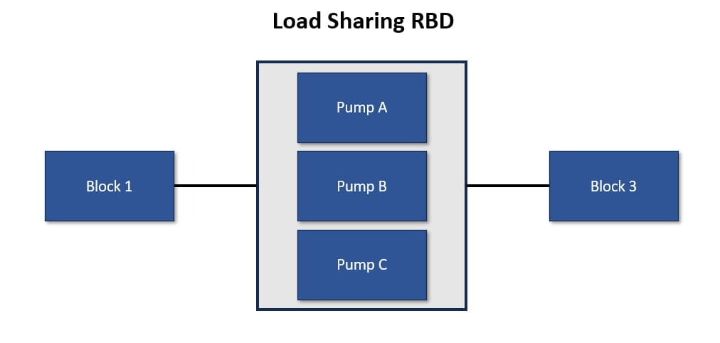
Load Sharing
Components share stress. Failure of one increases load on others. This is captured in a load sharing RBD.
Repairable Systems
Use Markov models or availability RBDs.
Practical Example: Data Center Power System
System:
- Two generators (parallel)
- One switchgear (series)
Reliability Functions
- Generators: Weibull
- Switchgear: Exponential
Results
| Time (hrs) | System Reliability |
|---|---|
| 1000 | 0.98 |
| 5000 | 0.85 |
| 10000 | 0.60 |
Insight
- Generators provide strong redundancy early
- Switchgear becomes the bottleneck over time
Software Tools
Several tools support time-dependent RBDs:
| Tool | Strength |
|---|---|
| ReliaSoft BlockSim | Advanced modeling |
| Minitab | Statistical analysis |
| Python (SciPy) | Custom modeling |
| MATLAB | Complex simulations |
When to Use Time-Dependent RBDs
Use them when:
- Systems degrade over time
- Maintenance matters
- Reliability targets depend on lifespan
- You need lifecycle insights
Avoid them when:
- Data is limited
- System is simple
- Time effects are negligible
Benefits in Six Sigma Projects
Time-dependent RBDs offer clear advantages:
- Better root cause analysis
- More accurate predictions
- Improved design decisions
- Optimized maintenance plans
They also support cost reduction by targeting high-impact improvements.
Example: Cost of Poor Reliability
| Failure Type | Cost per Event | Frequency | Annual Cost |
|---|---|---|---|
| Minor | $1,000 | 50 | $50,000 |
| Major | $10,000 | 10 | $100,000 |
Improving reliability over time reduces both frequency and cost.
Linking to COPQ (Cost of Poor Quality)
Reliability directly affects COPQ:
- Failures increase scrap
- Downtime reduces throughput
- Repairs increase labor costs
Time-dependent RBDs show when costs spike. That insight drives targeted improvements.
Conclusion
Time-dependent RBDs bring realism into reliability modeling. They reflect how systems behave in the real world. Components age. Failures cluster. Maintenance matters.
By adding time to RBDs, you unlock deeper insights. You move beyond static snapshots. Instead, you see the full lifecycle.
That perspective fits perfectly with Six Sigma. It supports data-driven decisions, highlights root causes, and drives sustainable improvement.
If you work on complex systems, you should not ignore time. Start simple. Build your first time-dependent RBD. Then refine it with real data.
Over time, your models will improve. More importantly, your systems will too.


